Summarising Data
Overview
Teaching: 30 min
Exercises: 5 minQuestions
What are the different types of variables?
What are measures of central tendency and variability?
Objectives
Define the different types of variables
Review measures of central tendency and variability
Review visualisation techniques such as box plots and histograms
Variable Types
Variables are the quantities measured in a sample. They may be classified as:
-
Quantitative i.e., numerical
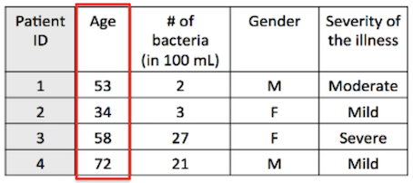
- Continuous (e.g., age, patient cholesterol levels)
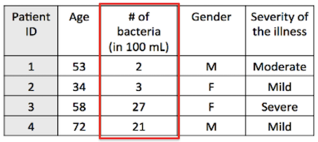
- Discrete (take a finite number of values)
-
Categorical
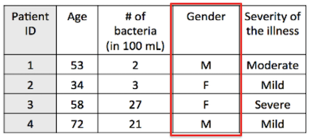
- Nominal (e.g., gender, blood group)
- Ordinal (ranked e.g., mild, moderate or severe illness)

Note: Often ordinal variables are re-coded to be quantitative.
Measures of Central Tendency and Variability
Numerical descriptive measures include:
- Measures of central tendency: Describe the centre of the distribution
- Measures of variability: Describe how the measurements vary about the centre of the distribution
Measures of central tendency
The mean is the sum of measurements divided by the total number of measurements.
If the data are arranged in increasing order, the median is:
- The middle value if n is an odd number, or
- The midway between the two middle values if n is an even number
The mode is the most commonly occurring value (value with the highest frequency).
Example: Calculating measures of central tendency
The systolic blood pressure readings of seven middle-aged men were as follows:
151, 124, 132, 170, 146, 124 and 113
Mean: \(\bar{x} = \frac{151 + 124 + 132 + 170 + 146 + 124 + 113}{7} = 137.14\)
Median: 113, 124, 124, 132, 146, 151, 170
Mode:
| 113 | 124 | 132 | 146 | 151 | 170 |
| 1 | 2 | 1 | 1 | 1 | 1 |
Measures of variability
Main measures of variability include:
- Range
- Variance
- Standard deviation
- Interquartile range (IQR)
The sample range is the difference between the largest and smallest observations in the sample.
This is useful for the “best” and “worst” case scenarios.
The sample variance, s², is the arithmetic mean of the squared deviations from the sample mean:
\[s^2 = \frac{\sum_{i=1}^{n}(x_i - \bar{x})^2}{n-1}\]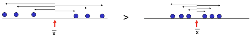
The sample standard deviation, s, is the square root of the variance.
Example: Calculating measures of variability
Using the blood pressure data (151, 124, 132, 170, 146, 124, 113):
Range: \(\text{Max} - \text{Min} = 170 - 113 = 57\text{mmHg}\)
Mean: \(\bar{x} = 137.14\)
Variance: \(s^2 = \frac{(151-137.14)^2 + (124-137.14)^2 + \cdots}{7-1} \approx 384.14\)
Standard deviation: \(s = \sqrt{384.14} \approx 19.60\)
Interquartile range
The median divides a distribution into two halves. The first and third quartiles (denoted Q₁ and Q₃) are defined as follows:
- 25% of the data lie below Q₁ (and 75% is above Q₁),
- 25% of the data lie above Q₃ (and 75% is below Q₃)
The interquartile range (IQR) is the difference between the first and third quartiles: IQR = Q₃ - Q₁.
Example: Calculating measures of variability - interquartile range
Using the blood pressure data (151, 124, 132, 170, 146, 124, 113):
Q1 = \(\frac{N}{4} = \frac{7}{4}= 1.75\)
Q3 = \(3 \times \frac{N}{4} = \frac{21}{4} = 5.25\)
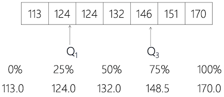
IQR = \(148.5 - 124 = 24.5\)
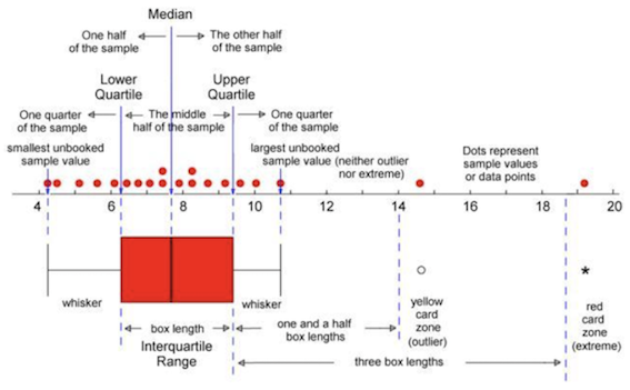
Box-Plots
A box-plot is a visual description of the distribution based on:
- Minimum
- Q1
- Median
- Q3
- Maximum
Box-plots are useful for comparing samples from several different treatments or populations.
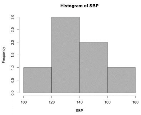
Histograms
A histogram is used to display the distribution of quantitative data in which the values are broken into a number of bins. The histogram is obtained by drawing rectangles in which the bases are the bin intervals and the heights are the counts in each bin.
Frequency histogram:
Relative frequency histogram:
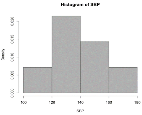
A relative frequency histogram represents the proportion of counts in each bin (total area of 1):
\(\text{height} = \frac{\text{count}}{\text{width} \times \text{total number}}\) → first one: \(\text{height} = \frac{1}{20 \times 7} \approx 0.007\)
Histograms are usually accompanied by a Probability Density Function, which is used for calculating the probabilities for continuous random variables and represents the density of probability for a continuous random variable over the specified ranges.
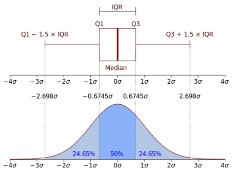
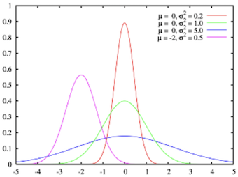
The Normal Distribution
Many variables of interest follow a normal distribution (e.g., age, height, weight, …). The normal distribution has a symmetric bell-shaped density curve, and is characterised by two parameters:
- Mean, µ
- Standard deviation, σ
X follows a normal distribution with the parameters μ (mean) and σ (standard deviation): \(X \sim N(\mu, \sigma)\)
Measures of variability: Which one to use?
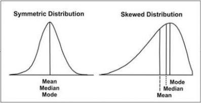
| Type of variable | Best measure of central tendency | Best measure of spread |
|---|---|---|
| Interval/ratio (not skewed) | Mean | Standard deviation |
| Interval/ratio (skewed) | Median | Range or interquartile range |
Tests for normality and variance equivalence
If our outcome variable is continuous and we are measuring it between two or more groups, then there are two additional tests that will need to be performed to help identify the most appropriate statistical test for the hypothesis.
- The Shapiro-Wilk test of normality
- The Levene’s test of equality of variances
Normal distribution: How to know?
To assess whether or not a random sample is selected from a normal distribution:
- Normal probability plot (quantile-quantile plot) to visualise the normality of the data
- Shapiro-Wilk test: H0: x1, …, xn are from a normally distributed population
Normal distribution: Transformation?
Sometimes data are non-normally distributed but may be log-normally distributed.
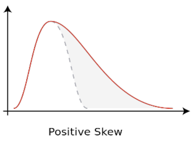
In the above image,
- The distribution is right-skewed
- The logarithm of the data is normal
The log-transformation of data is very common, mostly to eliminate skew in data.
Example:
Before log-transformation:
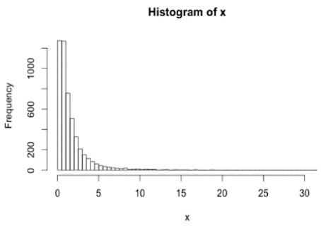
Shapiro-Wilk test results: p = 0.01 → non-normally distributed
After log transformation:
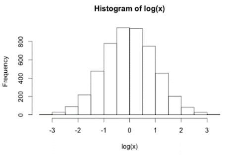
Shapiro-Wilk test results: p = 0.89 → normally distributed
Key Points
Understand the variable types referenced in this workshop
Understand how to calculate measures of central tendency and variability
Understand that box plots and histograms can be used to visualise data spread
Understand the normal distribution and why normality testing is an important step before conducting statistical comparisons