Comparison Between Two Groups
Overview
Teaching: 45 min
Exercises: 10 minQuestions
Do two sample groups differ for a continuous trait?
Objectives
Tests for use with comparison of two groups of continuous data
Summarising continuous data graphically
Selecting and using relevant statistical tests
Comparison of two sample groups
Earlier we discussed continuous data, and how to investigate relationships (correlations) between two continuous variables. In this section, we will learn how to identify whether a single continuous trait differs between two sample groups - a two sample test. Specifically, we will investigate whether there is a statistically-significant difference between the distribution of that variable between the two groups. As an example, we will test whether male patients in our gallstones study are taller than female patients.
Discussion
See if you can identify other examples where you might use a two sample groups comparison. Do you have any in your own research?
Choosing the relevant test
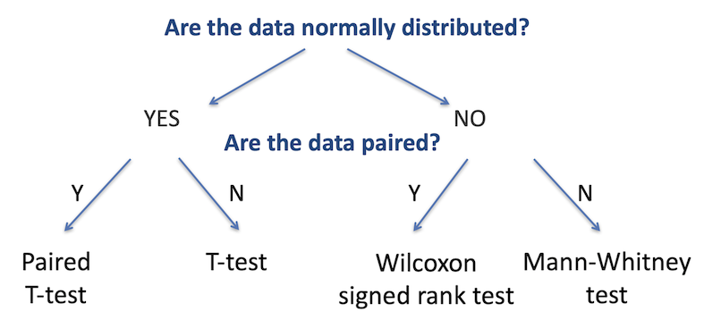
As with testing for categorical variables, there are a range of different statistical analyses for two sample group comparisons; the appropriate one to use is determined by the nature of the dataset. There are two primary questions we need to ask to identify the relevant test: are the two datasets normally-distributed, and are the data paired (that is, are there repeated measurements on the same samples)? The figure below summarises the choice of statistical test used for each of these cases.

The first step is to determine whether the continuous variable in each group is
normally distributed. We’ve already learned about the shapiro.test function to
test for normality, and can use that again in this situation.
The second decision is to identify whether the data is paired or not. Paired data is when the two groups are the same test samples but measured under different conditions (for example, a group of patients tested before and after treatment), unpaired is when the two groups are independent (for example, two separate groups of patients, one group treated and one untreated).
There are a few further subtleties beyond this which we will come to in a moment, but these are the two major determining factors in choosing the correct test.
Challenge 1
In our gallstones dataset, assume that BMI is normally distributed for patients with a recurrence of gallstones and not normal for those with no recurrence. Which test would we use to investigate whether those two groups (with and without recurrence) had different BMIs?
Solution to Challenge 1
One data set is normally distributed, the other is not, so we choose the option for non-normally distributed data - the branch to the right (we can only answer yes to the first question if both datasets are normal). The data is not paired - the patients with recurrence are a different group to those without. In this case we would use the Mann-Whitney test.
Two sample Student’s T-test
If data is normally distributed for both groups, we will generally use the Student’s T-test. This compares the means of two groups measured on the same continuous variable. Tests can be two-sided (testing whether the groups are not equal) or one-sided (testing either whether the second group is greater than or less that the first). As we discussed in the introduction, generally a two-sided test is preferred unless there is a specific reason why a single-sided one is justified.
H0: µ1 = µ2 | against | H1: µ1 ≠ µ2 (two-sided) | or | H0: µ1 <= µ2 | against | H1: µ1 > µ2 (greater) | or | H0: µ1 >= µ2 | against | H1: µ1 < µ2 (less)
If equal variance: Student’s T-test If unequal variance: Welch’s two-sample T-test If data are paired: Student’s paired T-test
Tip
The R
t.testfunction combines all three of these tests, and defaults to Welch’s two-sample T-test. To perform a standard T-test, use the parameter settingvar.equal = TRUE, and for a paired T-test, usepaired = TRUE.
Two sample Mann-Whitney test
Unless both groups are normally distributed, use the Mann-Whitney test. This is a non-parametric test analogous to the unpaired T-test, used when the dependent variable is non-normally distributed
The Mann-Whitney test compares the medians of the two groups rather than the means, by considering the data as rank order values rather than absolute values.
Tip
The
wilcox.testfunction in R defaults to unpaired data - effectively returning the Mann-Whitney test instead. Carry out a paired Wilcox test with thepaired = TRUEargument
Two sample test example
Is there a difference in height between females and males in the gallstones dataset?
Height: Continuous variable Gender: Categorical variable with two levels Null hypothesis: There is no difference in height between the groups
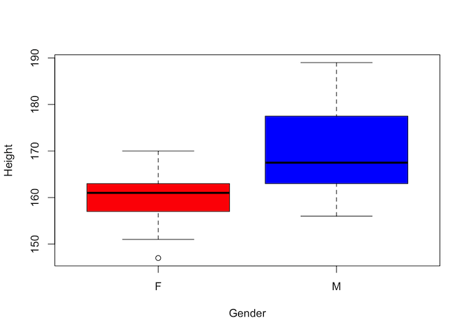
Step one - visualise the data We will start by reviewing the data using a boxplot to see if there is an indication of difference between the groups
plot(gallstones$Height ~ gallstones$Gender,
     col=c('red','blue'),
     ylab = 'Height',
     xlab = 'Gender')

Visually there certainly appears to be a difference. But is it statistically significant?
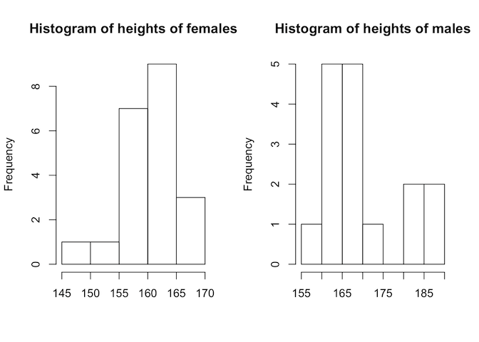
Step two - is the data normally distributed?
par(mfrow=c(1,2))
hist(gallstones$Height[which(gallstones$Gender == 'F')], main = "Histogram of heights of females", xlab = "")
hist(gallstones$Height[which(gallstones$Gender == 'M')], main = "Histogram of heights of males", xlab = "")
par(mfrow=c(1,1))

This doesn’t look very normally-distributed, but we do have relatively few data points. A more convincing way to determine this would be with the Shapiro-Wilks test
by(gallstones$Height, gallstones$Gender, shapiro.test)
## gallstones$Gender: F
##
## 	Shapiro-Wilk normality test
##
## data:  dd[x, ]
## W = 0.94142, p-value = 0.2324
##
## ------------------------------------------------------------
## gallstones$Gender: M
##
## 	Shapiro-Wilk normality test
##
## data:  dd[x, ]
## W = 0.88703, p-value = 0.05001
Neither test gives a significant p-value, so in the absence of sufficient evidence to accept the alternative hypothesis of non-normality, we treat the data as if it were normal; that is, we use a T-test
Step three - are variances equal?
# A quick and dirty test - how similar are the standard deviations?
by(gallstones$Height, gallstones$Gender, sd)
## gallstones$Gender: F
## [1] 5.518799
## ------------------------------------------------------------
## gallstones$Gender: M
## [1] 9.993331
# Or properly test for equality of variance using Levene's test
library(DescTools)
## Registered S3 method overwritten by 'DescTools':
##   method         from
##   reorder.factor gdata
LeveneTest(gallstones$Height ~ gallstones$Gender)
## Levene's Test for Homogeneity of Variance (center = median)
##       Df F value  Pr(>F)
## group  1  3.4596 0.07131 .
##       35
## ---
## Signif. codes:  0 '***' 0.001 '**' 0.01 '*' 0.05 '.' 0.1 ' ' 1
Although the standard deviations of the two groups (and hence the variances) seem to be quite different, Levene’s test gives a non-significant p-value of 0.07. This means that we shouldn’t reject the null hypothesis of equal variance, and so we should perform a Student’s T-test. If the variances had been different, then we would have used Welch’s two-sample T-test instead.
Step four - carry out a T-test
# Specify equal variance using the var.equal = TRUE argument.
# var.equal would be set to FALSE if the p-value of the Levene's test was less
# than 0.05, and the `t.test` function would then run a Welch's two-sample test.
t.test(gallstones$Height ~ gallstones$Gender, var.equal = TRUE)
##
## 	Two Sample t-test
##
## data:  gallstones$Height by gallstones$Gender
## t = -3.6619, df = 35, p-value = 0.00082
## alternative hypothesis: true difference in means is not equal to 0
## 95 percent confidence interval:
##  -14.655702  -4.201441
## sample estimates:
## mean in group F mean in group M
##        160.5714        170.0000
Conclusion: the p-value is significant so we can accept the alternative hypothesis and conclude that there is a difference in the mean height of males and females in our dataset.
Challenge 2
Using the gallstones dataset, test whether the gallstone diameter (“Diam”) is different between patients who suffer a recurrence and those who do not.
Solution to Challenge 2
# Visualise data
boxplot(gallstones$Diam ~ gallstones$Rec, col = c("red","blue"),
     ylab = "Diameter",
     xlab = "Recurrence")
# Test whether data is normally distributecd
by(gallstones$Diam, gallstones$Rec, hist)
by(gallstones$Diam, gallstones$Rec, shapiro.test)
Data is not normal for the recurrence group, and data is not paired - hence Mann-Whitney test
# Use wilcox.test function which defaults to Mann-Whitney analysis
wilcox.test(gallstones$Diam ~ gallstones$Rec)
The p-value is not significant, so we do not have sufficient evidence to reject the null hypothesis that there is no difference in gallstone size between the two groups.
Group descriptions
If there is a significant difference between the two groups (or even if there
isn’t) it is often useful to generate some summary statistics for each group.
We can do this with the by command, which we’ve used already in this section,
combined with summary functions
# For normally distributed data, report the mean and standard deviation
by(gallstones$Height, gallstones$Gender, mean)
## gallstones$Gender: F
## [1] 160.5714
## ------------------------------------------------------------
## gallstones$Gender: M
## [1] 170
by(gallstones$Height, gallstones$Gender, sd)
## gallstones$Gender: F
## [1] 5.518799
## ------------------------------------------------------------
## gallstones$Gender: M
## [1] 9.993331
# For non-normally distributed data, report the median and inter-quartile range
by(gallstones$Diam, gallstones$Rec, median)
## gallstones$Rec: NoRecurrence
## [1] 10
## ------------------------------------------------------------
## gallstones$Rec: Recurrence
## [1] 8.5
by(gallstones$Diam, gallstones$Rec, IQR)
## gallstones$Rec: NoRecurrence
## [1] 12
## ------------------------------------------------------------
## gallstones$Rec: Recurrence
## [1] 9
# Many of the summary statistics can be calculated in one step with the FSA
# Summarize function
library(FSA)
Summarize(gallstones$Height~gallstones$Gender)
##   gallstones$Gender  n     mean       sd min  Q1 median     Q3 max
## 1                 F 21 160.5714 5.518799 147 157  161.0 163.00 170
## 2                 M 16 170.0000 9.993331 156 164  167.5 175.25 189
Summarize(gallstones$Diam~gallstones$Rec)
##   gallstones$Rec  n     mean       sd min Q1 median Q3 max
## 1   NoRecurrence 21 12.42857 7.440238   3  6   10.0 18  27
## 2     Recurrence 16 10.06250 6.180278   4  5    8.5 14  26
Paired samples
If data is paired, that is, it is the same samples under two different conditions, we can take advantage of that to carry out statistical tests with greater discriminatory power. That is because by using paired samples, we remove a lot of the noise that can otherwise obscure our results. Paired data must have the same number of results in each group, there must be a one-to-one relationship between the groups (every sample that appears in one group must appear in the other), and the data must be the same sample order in each group.
Otherwise, paired sample analysis is performed in a similar way to unpaired
analysis. The main difference is to add the paired = TRUE argument to the
t.test or wilcox.test function.
Key Points
Use
histand boxplots to review distribution of variables for a groupSummarise grouped data using the
bycommandDistinguish paired and non-paired samples
Correctly use the
t.testandwilcox.testfunctions