Testing For More Than Two Groups

Overview

Teaching: 45 min
Exercises: 10 min

Questions

Are the group means different among three or more groups?

Objectives

Identify situations needing multiple sample tests and choose the correct test for the type of data

Perform one and two-way ANOVA testing

Recognise interaction effects in multiple-category testing

Interpret test results and apply post hoc testing

Comparison of multiple groups

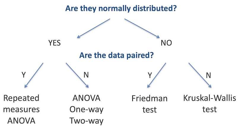
The T-test, Mann-Whitney Test and others discussed earlier are designed to identify differences in the means or medians of two groups. When working with data that is in three or more groups, where we are testing if there is a difference between any one of those groups with the others, we need to use other tests. As with two-sample testing, the appropriate test is determined in large part by whether the data in each group is normally distributed, and whether the data is paired, as outlined in the figure below.

RStudio layout

Challenge 1

Based on what you have learned previously in this workshop, how can we best determine whether the data in each sample is normally distributed
Solution to Challenge 1

We can use the shapiro.test function to test for normality - or rather, to test the alternative hypothesis that the data is not normally distributed. Use the by function to test all categories in one command:
by(data$measurement, data$category, shapiro.test)
Remember, as with the two sample tests, if any one group is not normally distributed, the whole analysis must be performed with the relevant non-parametric test

ANOVA Testing - One-way

The one-way ANOVA compares whether there is a difference in the mean values of three or more groups. It requires one continuous (and normally distributed) measurement variable, and one categorical variable (with three or more categories).

Assumptions for the one-way ANOVA are:

Independant samples
Normal distribution in each group
Homogeneity of variances

The null hypothesis for one-way ANOVA is that the means of all groups are equal; the alternative hypothesis is that at least one of the means is different from the others.

H₀: µ₁ = µ₂ = µ₃ = … = µ_k H₁: µ₁ ≠ µ₂ OR µ₁ ≠ µ₃ OR µ₂ ≠ µ₃ ….

The ANOVA extension of the t-test is called the F-test, and is based around decomposing the total variation in the sample into the variability (sum of squares) within groups and between groups

RStudio layout

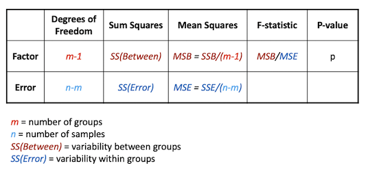
ANOVA one-way example

In our example dataset, the alcohol consumption field has three categories. We will test if there is any effect on weight associated with the alcohol consumption category.

Variables of interest

Alcohol consumption: Categorical (1, 2 or 3)
Weight: Continuous

There are two variables - one categorical with more than two levels and one continuous. The data are not paired - all the measurements are from different patients. So based on the decision tree, the appropriate test is either one-way ANOVA or Kruskal-Wallis test. The choice between these is made depending on whether the data is normally distributed or not

table(gallstones$Alcohol.Consumption)

##
## NonAlcohol   Previous    Alcohol
##          9         10         18

by(gallstones$Weight, gallstones$Alcohol.Consumption, shapiro.test)

## gallstones$Alcohol.Consumption: NonAlcohol
##
## 	Shapiro-Wilk normality test
##
## data:  dd[x, ]
## W = 0.79876, p-value = 0.01976
##
## ------------------------------------------------------------
## gallstones$Alcohol.Consumption: Previous
##
## 	Shapiro-Wilk normality test
##
## data:  dd[x, ]
## W = 0.95864, p-value = 0.7703
##
## ------------------------------------------------------------
## gallstones$Alcohol.Consumption: Alcohol
##
## 	Shapiro-Wilk normality test
##
## data:  dd[x, ]
## W = 0.94549, p-value = 0.3588

The Shapiro test for group 1 gives a significant p-value, indicating that we should reject the null hypothesis that the data is normally distributed. This would indicate that the Kruskal-Wallis test is the appropriate one for this analysis

kruskal.test(gallstones$Weight ~ gallstones$Alcohol.Consumption)

##
## 	Kruskal-Wallis rank sum test
##
## data:  gallstones$Weight by gallstones$Alcohol.Consumption
## Kruskal-Wallis chi-squared = 0.89142, df = 2, p-value = 0.6404

boxplot(gallstones$Weight ~ gallstones$Alcohol.Consumption)

RStudio layout

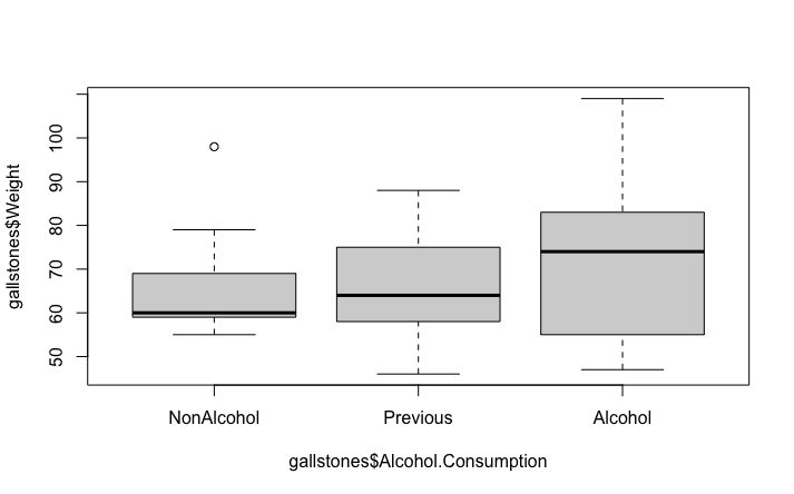
We can see that with a p-value of 0.64, we reject the alternative hypothesis and concluded that in this data set, there is no evidence for a difference in patient weight associated with their level of alcohol consumption. This is consistent with the plot, which doesn’t show any clear differences between the three categories.

For comparison and practice, let’s also perform an ANOVA

result <- aov(gallstones$Weight~gallstones$Alcohol.Consumption)
summary(result)

##                                Df Sum Sq Mean Sq F value Pr(>F)
## gallstones$Alcohol.Consumption  2    369   184.4   0.685  0.511
## Residuals                      34   9151   269.1

Like the Kruskal-Wallis test, this ANOVA also gives a non-significant p-value, but remember, it is not the appropriate test for non-normally distributed data so would not be a valid test anyway.

Post-Hoc testing

The one-way ANOVA and Kruskal-Wallis tests only identify that one (or more) of the groups has a significant difference to the others. To go further, we would want to identify which group(s) were different. For this we would use a Post-hoc test, either Tukeys’ HSD for ANOVA or Dunn’s test (in the FSA package) for Kruskal-Wallis. This performs a multiple-testing corrected pairwise comparison between each combination of groups to highlight which (if any) are different.

# Dunn's test, since we used Kruskal-Wallis for the initial analysis
dunnTest(gallstones$Weight~gallstones$Alcohol.Consumption, method = "bonferroni")

## Dunn (1964) Kruskal-Wallis multiple comparison

##   p-values adjusted with the Bonferroni method.

##              Comparison           Z   P.unadj P.adj
## 1  Alcohol - NonAlcohol  0.79245283 0.4280967     1
## 2    Alcohol - Previous  0.75516608 0.4501493     1
## 3 NonAlcohol - Previous -0.05588197 0.9554358     1

The output shows a pairwise comparison and associated p-value for each combination of the groups being tested - groups 2 and 1 first, then groups 3 and 1, and finally groups 3 and 2. In this example, the p-values are all 1 - there is not evidence for even the slightest difference between the groups!

If there is a significant p-value with a one-way ANOVA, use the Tukey HSD test

TukeyHSD(result)

##   Tukey multiple comparisons of means
##     95% family-wise confidence level
##
## Fit: aov(formula = gallstones$Weight ~ gallstones$Alcohol.Consumption)
##
## $`gallstones$Alcohol.Consumption`
##                           diff       lwr      upr     p adj
## Previous-NonAlcohol -0.2777778 -18.74892 18.19336 0.9992516
## Alcohol-NonAlcohol   6.1666667 -10.24537 22.57870 0.6311298
## Alcohol-Previous     6.4444444  -9.41109 22.29998 0.5844049

The layout here is similar to the Dunn’s test with one row per comparison and the p-value reported for each pairwise comparison

Challenge 2

For a more interesting analysis, try creating a dummy dataset with the weight of patients doubled for just one category of Alcohol.Consumption and then repeat the Kruskal-Wallis and Dunn’s tests. Does this show a significant difference as you might expect?
Solution to Challenge 2
# Create a copy of the gallstones data frame so as not to break things later
dummy_data <- gallstones
# Double the weight for Alcohol.Consumption category 'Alcohol'
ac_three <- which(gallstones$Alcohol.Consumption == 'Alcohol')
dummy_data[ac_three, "Weight"] <- 2 * dummy_data[ac_three, "Weight"]
# Then do the testing
kruskal.test(dummy_data$Weight ~ dummy_data$Alcohol.Consumption)
dunnTest(dummy_data$Weight~dummy_data$Alcohol.Consumption,
                   method = "bonferroni")

Challenge 3

Try using the dummmy dataset from challenge 2 for an ANOVA and Tukey’s test
Solution to Challenge 3
dummy_result <- aov(dummy_data$Weight ~ dummy_data$Alcohol.Consumption)
summary(dummy_result)
TukeyHSD(dummy_result)

ANOVA Testing - Two-way

An alternative application of ANOVA testing is where there are two categorical variables (or factors) and one continuous measurement variable. This is commonly used where the effect of a treatment or intervention might be different between subsets of the test population - in other words, where there is a possibility of an interaction between the two factors. A common situation might be a different response of male and female patients to a drug treatment, which is the example that we will use here.

Two-way ANOVA example

The dataset we will use here is a small study to investigate the influence of Prozac on the reported ‘happiness score’ of patients, and whether males and female patients respond differently.

Happiness score recorded for 24 patients
Patients randomised to either placebo or Prozac treatment (first factor)
Patients gender recorded (second factor)

Read the data in from the file “happiness.csv”

# As before, we need to specify the stringsAsfactors flag for read.csv
happiness <- read.csv("data/happiness.csv", stringsAsFactors = TRUE)
head(happiness)

##   Patient Score Gender Treatment
## 1       1     3   Male   Placebo
## 2       2     4   Male   Placebo
## 3       3     2   Male   Placebo
## 4       4     3   Male   Placebo
## 5       5     4   Male   Placebo
## 6       6     3   Male   Placebo

str(happiness)

## 'data.frame':	24 obs. of  4 variables:
##  $ Patient  : int  1 2 3 4 5 6 7 8 9 10 ...
##  $ Score    : num  3 4 2 3 4 3 4 5 4 6 ...
##  $ Gender   : Factor w/ 2 levels "Female","Male": 2 2 2 2 2 2 1 1 1 1 ...
##  $ Treatment: Factor w/ 2 levels "Placebo","Prozac": 1 1 1 1 1 1 1 1 1 1 ...

summary(happiness)

##     Patient          Score          Gender     Treatment
##  Min.   : 1.00   Min.   :2.000   Female:12   Placebo:12
##  1st Qu.: 6.75   1st Qu.:4.000   Male  :12   Prozac :12
##  Median :12.50   Median :5.000
##  Mean   :12.50   Mean   :4.854
##  3rd Qu.:18.25   3rd Qu.:6.000
##  Max.   :24.00   Max.   :7.000

table(happiness$Gender, happiness$Treatment)

##
##          Placebo Prozac
##   Female       6      6
##   Male         6      6

This corresponds to this design:

RStudio layout

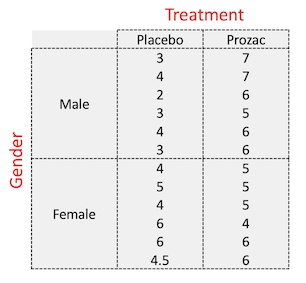
As usual, an early step in studying our data is to visualise it

# First, plot just using each of the factors independently
par(mfrow=c(1,2))
plot(Score ~ Treatment + Gender, data = happiness)
par(mfrow=c(1,1))

RStudio layout

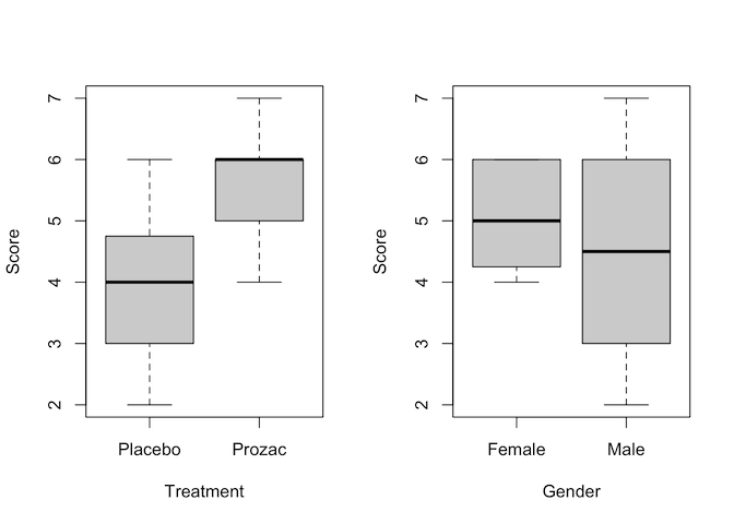
# Then using ggplot to separate out the four different combinations of factor
ggplot(data = happiness, aes(x = Treatment, y = Score, fill = Gender)) +
  geom_boxplot(position = position_dodge())

RStudio layout

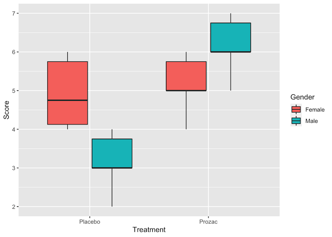
Judging by the boxplots, there appears to be a difference in happiness score for the different treatment drugs (score higher with treatment than placebo). However, the difference is less pronounced between the gender groups.

Two-way ANOVA tests for two things: Main effects - each factor independently

Are patients happier on placebo or Prozac
Do males and females differ in happiness score

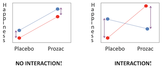
Interaction effects - the effects of one factor are different depending on the level (category) of the other factor

Treatment x Gender: Males may be happier on Prozac than placebo, but females may not have a different response between the two. Or vice versa. The diagram below shows examples of (left) where both main effects have a difference but there is no interaction and (right) where there is a strong interaction but little main effect.

RStudio layout

Interaction plots can be made in R using the interaction.plot command. Note the order of factors - switching these alters which variable is plotted on the x-axis.

interaction.plot(happiness$Treatment, happiness$Gender, happiness$Score,
                 col=2:3, lwd=3)

RStudio layout

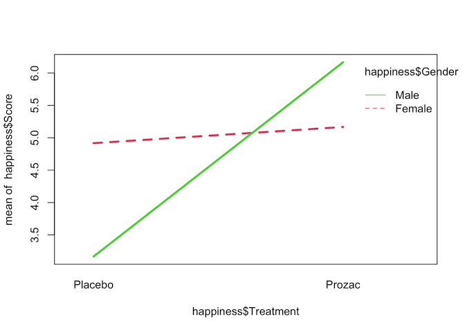
The interaction plot seems to show that there is a strong interaction effect between Treatment and Gender on happiness score, but to confirm that we can fit a two-way ANOVA with an interaction term.

# Option 1 - the most commonly used
result <- aov(Score~Treatment+Gender+Treatment*Gender, data=happiness)
summary(result)

##                  Df Sum Sq Mean Sq F value   Pr(>F)
## Treatment         1 15.844  15.844  24.934 6.98e-05 ***
## Gender            1  0.844   0.844   1.328 0.262773
## Treatment:Gender  1 11.344  11.344  17.852 0.000415 ***
## Residuals        20 12.708   0.635
## ---
## Signif. codes:  0 '***' 0.001 '**' 0.01 '*' 0.05 '.' 0.1 ' ' 1

# Option 2 - gives identical results under most circumstances
result_2 <- lm(Score~Treatment+Gender+Treatment*Gender, data=happiness)
anova(result_2)

## Analysis of Variance Table
##
## Response: Score
##                  Df  Sum Sq Mean Sq F value    Pr(>F)
## Treatment         1 15.8437 15.8437 24.9344 6.977e-05 ***
## Gender            1  0.8437  0.8437  1.3279 0.2627729
## Treatment:Gender  1 11.3437 11.3437 17.8525 0.0004155 ***
## Residuals        20 12.7083  0.6354
## ---
## Signif. codes:  0 '***' 0.001 '**' 0.01 '*' 0.05 '.' 0.1 ' ' 1

Interpretation of two-way ANOVA output

Treatment

The final column Pr(>F) is the p-value; at 7x10^-5 this is well within the cutoff for statistical significance. Therefore we conclude that treatment with Prozac has a significant effect on happiness. From our plots it appears that Prozac is associated with higher happiness scores, but this should be confirmed with post hoc testing.

Gender

The p-value for gender is not signficant, so there is not evidence for a gender effect on happiness; that is, there is no difference in happiness levels between males and females.

Treatment:Gender

This has a significant p-value, indicating that there is an interaction between gender and treatment. The plots suggest that is because Prozac increases happiness in men more than in women, but again this should be confirmed with post hoc testing.

# For ANOVA performed with `aov()`, used TukeyHSD for post hoc testing
result <- aov(Score~Treatment+Gender+Treatment*Gender, data=happiness)
TukeyHSD(result)

##   Tukey multiple comparisons of means
##     95% family-wise confidence level
##
## Fit: aov(formula = Score ~ Treatment + Gender + Treatment * Gender, data = happiness)
##
## $Treatment
##                 diff       lwr      upr    p adj
## Prozac-Placebo 1.625 0.9461711 2.303829 6.98e-05
##
## $Gender
##               diff       lwr       upr     p adj
## Male-Female -0.375 -1.053829 0.3038289 0.2627729
##
## $`Treatment:Gender`
##                               diff         lwr        upr     p adj
## Prozac:Female-Placebo:Female  0.25 -1.03813584  1.5381358 0.9472984
## Placebo:Male-Placebo:Female  -1.75 -3.03813584 -0.4618642 0.0056547
## Prozac:Male-Placebo:Female    1.25 -0.03813584  2.5381358 0.0591502
## Placebo:Male-Prozac:Female   -2.00 -3.28813584 -0.7118642 0.0016445
## Prozac:Male-Prozac:Female     1.00 -0.28813584  2.2881358 0.1650724
## Prozac:Male-Placebo:Male      3.00  1.71186416  4.2881358 0.0000132

The $Treatment section of this output supports our conclusion from the two-way ANOVA that Prozac increases happiness score, by an average of 1.6 happiness units (95% CI: 0.95-2.3). The $Treatment:Gender section indicates that Prozac has no effect on happiness in females (or at least, not a statistically signficant effect), but in males it increases happiness by approximatey 3.0 units.

Checking assumptions

After fitting an ANOVA model it is important to always check the relevant model assumptions. This includes making QQ-plots and residual plots

par(mfrow=c(2,2))
plot(result)

RStudio layout

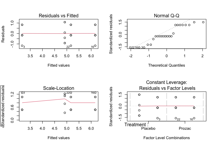
Characteristics of a well-behaved residual vs. fits plot

The residuals “bounce randomly” around the 0 line. This suggests that the assumption that the relationship is linear is reasonable.
The residuals roughly form a “horizontal band” around the 0 line. This suggests that the variances of the error terms are equal.
No one residual “stands out” from the basic random pattern of residuals. This suggests that there are no outliers.

Characteristics of a well-behaved Q-Q plot

If the points on the q-q plot fall approximately on a straight line, the residuals are considered to be normally distributed.
If some points are far from the line have a deeper look to see if they are outliers.

In this case, it appears that there is a deviation from normality because many of the points do not fall on the straight line.

Scale location plot

Square root of the standardized residuals (sort of a square root of relative error) as a function of the fitted values. Again, there should be no obvious trend in this plot.

Point Leverage plot

Measure of importance of each point in determining the regression result. Superimposed on the plot are contour lines for the Cook’s distance (another measure of the importance of each observation).

Smaller distances means that removing the observation has little affect on the regression results. Distances larger than 2 are suspicious and suggest the presence of a possible outlier.

Paired data with more than two samples

The two-way ANOVA and Kruskal-Wallis test are both intended for use with independent sets of data, as outlined in the decision tree at the start of this section. As with several other tests we have explored in this course, there are alternatives that should be used when data points are paired - in other words, where there are multiple measurements on the same subject. These are the Repeated measures ANOVA and the Friedman test, for normally distributed and non-normally distributed data respectively.

Typical study designs where you might use paired data analysis approaches include:

Studies that investigate changes in mean scores over three or more time points
Studies that investigate differences in mean scores under three or more different conditions.

These more advanced tests are beyond the scope of this workshop, but some are covered in our Longitudinal and Mixed Model Analysis course.

Challenge 4

Can you think of a modification to our Happiness trial example which would mean it should be analysed using a paired data technique?

Solution to Challenge 4

One option would be that if, rather than testing on 24 individuals assigned randomly to placebo/treatment groups, the trial was instead carried out with 12 people and happiness scores recorded before and after treatment with Prozac. Or perhaps a stricter design - 24 individuals treated with either Prozac or placebo, with happiness scores recorded before and after treatment.

Key Points

Identify situations needing multiple sample tests and choose the relevant test using the decision tree

Perform multi-group testing using aov and kruskal.test

Perform and interpret post hoc tests using TukeyHSD and dunn.test

Study interactions using interaction.plot and aov

Check model assumptions using plot

previous episode

Statistical Comparisons using R

next episode

Testing For More Than Two Groups

Overview

Comparison of multiple groups

Challenge 1

Solution to Challenge 1

ANOVA Testing - One-way

ANOVA one-way example

Variables of interest

Post-Hoc testing

Challenge 2

Solution to Challenge 2

Challenge 3

Solution to Challenge 3

ANOVA Testing - Two-way

Two-way ANOVA example

Interpretation of two-way ANOVA output

Treatment

Gender

Treatment:Gender

Checking assumptions

Characteristics of a well-behaved residual vs. fits plot

Characteristics of a well-behaved Q-Q plot

Scale location plot

Point Leverage plot

Paired data with more than two samples

Challenge 4

Solution to Challenge 4

Key Points

previous episode

next episode