Categorical Variables
Overview
Teaching: 45 min
Exercises: 10 minQuestions
What is a categorical variable?
What statistical tests are used with categorical data?
Objectives
Tests for use with categorical variables
Summarising categorical data with barcharts
Using factors to code categorical variables
Introducing categorical data
Having looked at the gallstones dataset, you will have noticed that many of the columns contain just two or three distinct values - for example, M and F, or 1, 2, and 3. These are examples of categorical data - where samples are assigned to one of a limited number of fixed, distinct categories. Categories may be emergent features of the data (for example ‘received treatment’ and ‘did not receive treatment’) but others may be more arbitrary according to the needs of the analysis (in this dataset, the three levels of alcohol consumption relate to ‘no consumption’, ‘previous consumer’ and ‘current consumer’).
Because categorical data typically has no intrinsic ordering to the categories, we cannot study relationships between two variables by looking for correlations. Instead, statistical analysis of categorical data is based around count frequencies - are the numbers of samples in each category what would be expected from random distribution, or do certain categories occur together more often than would happen just by chance?
Ordinal data
An intermediate between categorical data and continuous data is ordinal data. Unlike categorical data, ordinal data does have natural order to the categories, but samples are still assigned to one of a fixed number of categories. For example, it is common on survey forms to see an ordinal age field: under 15, 15-25, 26-40, etc. Ordinal data is outside the scope of today’s workshop - talk to a statistician if you need more advice.
Challenge 1
Look again at the gallstones dataset. How many categorical fields does it contain?
Solution to Challenge 1
There are seven categorical fields in this dataset: Gender, Obese, Smoking.Status, Alcohol.Consumption, Treatment, Rec, and Mult
Using factors for categorical data
With the exception of Gender, all the categorical variables in the gallstones dataframe have been recorded as integer fields. This may cause confusion because it would be possible in principle to analyse these as continuous variables. R includes the factor data type, which provides a way to store a fixed, predefined set of values. This makes it ideal for working with categories, so we will convert those columns to factors.
# Either convert the columns one at a time
gallstones$Obese <- as.factor(gallstones$Obese) # and repeat for other five
# Or all together: variables Obese to Mult (columns 7-12) need to be categorical
gallstones[,7:12] <- data.frame(lapply(gallstones[,7:12], as.factor))

# While we're at it, convert the levels to meaningful category names
levels(gallstones$Obese) <- c("NonObese", "Obese")
levels(gallstones$Treatment) <- c("Untreated", "Treated")
levels(gallstones$Rec) <- c("NoRecurrence", "Recurrence")
levels(gallstones$Smoking.Status)<-c("NonSmoker","Smoker")
levels(gallstones$Alcohol.Consumption)<-c("NonAlcohol","Previous","Alcohol")
levels(gallstones$Mult)<-c("Single","Multiple")
str(gallstones)
## 'data.frame':	37 obs. of  14 variables:
##  $ Patient_ID         : chr  "P25" "P28" "P17" "P27" ...
##  $ Gender             : Factor w/ 2 levels "F","M": 1 1 2 1 1 1 1 1 1 1 ...
##  $ Age                : int  64 81 77 80 86 69 75 77 73 88 ...
##  $ Height             : int  147 151 156 156 156 157 157 160 160 160 ...
##  $ Weight             : int  65 69 59 47 53 48 46 55 51 54 ...
##  $ BMI                : num  30.1 30.3 24.2 19.3 21.8 ...
##  $ Obese              : Factor w/ 2 levels "NonObese","Obese": 2 2 1 1 1 1 1 1 1 1 ...
##  $ Smoking.Status     : Factor w/ 2 levels "NonSmoker","Smoker": 2 2 2 2 2 1 2 2 2 1 ...
##  $ Alcohol.Consumption: Factor w/ 3 levels "NonAlcohol","Previous",..: 1 2 1 3 2 3 2 3 3 3 ...
##  $ Treatment          : Factor w/ 2 levels "Untreated","Treated": 2 1 1 2 1 2 1 2 1 2 ...
##  $ Rec                : Factor w/ 2 levels "NoRecurrence",..: 2 2 1 1 2 1 2 1 2 1 ...
##  $ Mult               : Factor w/ 2 levels "Single","Multiple": 2 2 1 1 1 1 2 1 1 2 ...
##  $ Diam               : int  6 7 20 15 18 19 14 18 15 5 ...
##  $ Dis                : int  8 6 20 2 14 8 8 4 15 3 ...
Visualising categorical data
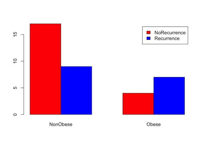
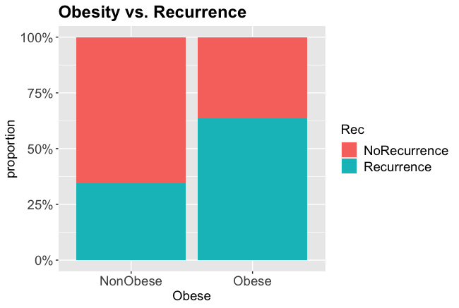
As with continuous data, it can often be useful to visualise categorical data before starting on more complex analysis. We can do this numerically with a simple count table, or graphically by expressing that table as a bar graph. For this example, we will test whether there is a relationship between obesity and the recurrence of gallstones.
# Summarise the data into a table.
counts <- table(gallstones$Rec, gallstones$Obese)
counts
##
##                NonObese Obese
##   NoRecurrence       17     4
##   Recurrence          9     7
addmargins(counts)
##
##                NonObese Obese Sum
##   NoRecurrence       17     4  21
##   Recurrence          9     7  16
##   Sum                26    11  37
# Displaying as proportions may be easier to interpret than counts
round(prop.table(table(gallstones$Rec, gallstones$Obese), margin = 2)*100,2)
##
##                NonObese Obese
##   NoRecurrence    65.38 36.36
##   Recurrence      34.62 63.64
Obese patients had a 63.6% chance of recurrence, non-obese patients only 34.6%
# Plots are generally easier to interpret than tables, so review data as a
# bar graph
barplot(counts, beside=TRUE, legend=rownames(counts), col = c('red','blue'))

# ggplot can be used for higher quality figures, and to plot proportions rather
# than counts
ggplot(gallstones, aes(Obese, fill=Rec)) +
  geom_bar(position="fill") +
  scale_y_continuous(labels=scales::percent) +
  theme(axis.text=element_text(size=14),
        legend.text=element_text(size=14),
        legend.title=element_text(size=14),
        axis.title=element_text(size=14),
        plot.title = element_text(size=18, face="bold")) +
  ylab("proportion") +
  ggtitle("Obesity vs. Recurrence")

From the charts and table it certainly looks like obesity is associated with a higher rate of recurrence, so we will test whether that is statistically significant.
Statistical tests for categorical variables
To carry out a statistical test, we need a null and alternative hypothesis. In most cases, the null hypothesis H0 is that the proportion of samples in each category is the same in both groups.
Our question: Is there a relationship between obesity and gallstone recurrence?
Hypotheses: H0: Gallstone recurrence is independent of obesity H1: Gallstone recurrence is linked with obesity
There are three main hypothesis tests for categorical variables:
- Chi-square test
chisq.test(): used when the expected count in each cell of the table is greater than 5 - Fisher’s exact test
fisher.test(): used when the expected count of at least one cell is ≤ 5 - McNemar test
mcnemar.test(): used for paired data - for example, the proportion of patients showing a particular symptom before and after treatment
Which test do we need? The data is not paired, so it is not the McNemar test. What are the expected counts for each cell?
# CrossTable from gmodels library gives expected counts, and also proportions
library(gmodels)
CrossTable(gallstones$Rec, gallstones$Obese,
           format = "SPSS", expected = T, prop.chisq = F)
## Warning in chisq.test(t, correct = TRUE, ...): Chi-squared approximation may be
## incorrect

## Warning in chisq.test(t, correct = FALSE, ...): Chi-squared approximation may be
## incorrect

##
##    Cell Contents
## |-------------------------|
## |                   Count |
## |         Expected Values |
## |             Row Percent |
## |          Column Percent |
## |           Total Percent |
## |-------------------------|
##
## Total Observations in Table:  37
##
##                | gallstones$Obese
## gallstones$Rec | NonObese  |    Obese  | Row Total |
## ---------------|-----------|-----------|-----------|
##   NoRecurrence |       17  |        4  |       21  |
##                |   14.757  |    6.243  |           |
##                |   80.952% |   19.048% |   56.757% |
##                |   65.385% |   36.364% |           |
##                |   45.946% |   10.811% |           |
## ---------------|-----------|-----------|-----------|
##     Recurrence |        9  |        7  |       16  |
##                |   11.243  |    4.757  |           |
##                |   56.250% |   43.750% |   43.243% |
##                |   34.615% |   63.636% |           |
##                |   24.324% |   18.919% |           |
## ---------------|-----------|-----------|-----------|
##   Column Total |       26  |       11  |       37  |
##                |   70.270% |   29.730% |           |
## ---------------|-----------|-----------|-----------|
##
##
## Statistics for All Table Factors
##
##
## Pearson's Chi-squared test
## ------------------------------------------------------------
## Chi^2 =  2.652483     d.f. =  1     p =  0.1033883
##
## Pearson's Chi-squared test with Yates' continuity correction
## ------------------------------------------------------------
## Chi^2 =  1.601828     d.f. =  1     p =  0.2056444
##
##
##        Minimum expected frequency: 4.756757
## Cells with Expected Frequency < 5: 1 of 4 (25%)
This is slightly complicated output, but we are most interested in the “Expected Values” and “Column Percent” figures - the second and fourth line of each box. These show:
- The expected number of obese patients suffering recurrence is 4.757 (<5)
- The recurrence rate in non-obese patients is 34.6%, whereas in obese patients it is 63.6%
Because one expected value is less than 5, we should use Fisher’s Exact test
fisher.test(gallstones$Obese, gallstones$Rec)
##
## 	Fisher's Exact Test for Count Data
##
## data:  gallstones$Obese and gallstones$Rec
## p-value = 0.1514
## alternative hypothesis: true odds ratio is not equal to 1
## 95 percent confidence interval:
##   0.6147706 19.2655239
## sample estimates:
## odds ratio
##   3.193654
Perhaps surprisingly given the plot data, the p-value of this test is not significant; this means that there is insufficient evidence to conclude that there is any difference in recurrence rates between obese and non-obese patients. The apparently higher rate of recurrence in obese patients is no more than might be expected by random chance in a sample group of this size. It is possible however that we have made a type II error and incorrectly failed to reject H0 - we should have consulted a statistician before gathering the data to check whether the sample size provided sufficient statistical power to detect a relationship.
Challenge 2
When would you use the Chi-square test
- When one variable is categorical and the other continuous
- When there is categorical data with more than five counts expected in each cell
- When there is paired categorical data
- You can use it interchangeably with Fisher’s Exact test
Solution to Challenge 2
Answer: 2
Challenge 3
Repeat the analysis to test whether recurrence is affected by treatment.
Prepare simple and proportion/expected tables, prepare a bar chart, identify and perform the appropriate statistical test.
Solution to Challenge 3
# Create the initial counts table
counts2 <- table(gallstones$Rec, gallstones$Treatment)
counts2

# Plot using barplot
barplot(counts2, beside = TRUE, legend = rownames(counts2),
        col = c('red','blue'))
# Or plot using ggplot
ggplot(gallstones, aes(Treatment, fill=Rec)) +
  geom_bar(position="fill") +
  scale_y_continuous(labels=scales::percent) +
  theme(axis.text=element_text(size=14),
        legend.text=element_text(size=14),
        legend.title=element_text(size=14),
        axis.title=element_text(size=14),
        plot.title = element_text(size=18, face="bold")) +
  ggtitle("Treatment vs. Recurrence")

# Look at expected values to select Chi-square or Fisher's Exact
library(gmodels) # Optional if the library is already installed
CrossTable(gallstones$Treatment,gallstones$Rec,format="SPSS",prop.chisq=F,expected=T)

# All expected values are greater than 5
chisq.test(gallstones$Treatment, gallstones$Rec, correct=FALSE)
Again, despite the barplot suggesting an association, the p-value is non-significant, so we reject the alternative hypothesis that treatment has an effect on recurrence rate
Key Points
Convert dataframe columns to factors using
as.factorDraw barcharts using
plotandggplotSelect an appropriate statistical test for a categorical dataset
Analyse categorical data using
chisq.testandfisher.test